Introduction

The purpose of our pipeline is to coregister neuroimaging datasets of different modalities and with different coordinate systems. We support 3D to 3D mapping, 3D to 2D mapping (e.g. mapping to serial sections), and 2D to 2D mapping (e.g. rigidly aligning slices with different stains).

We perform registration using diffeomorphisms (with time varying velocity field parameterization) and affine transforms. These transformations can be composed to map data between coordinate spaces and between single specimens and common coordinate systems.

Examples of typical workflows are below. In the diagrams below, each arrow represents the computation of a transformation. By following arrows in the forward or reverse direction, all data can be reconstructed in any of the available spaces. A minor caveat is that only low resolution 2D summary data can be reconstructed in a 3D space.

Example workflow: STP mapping

A common setting is when we do not have serial section data. For example we may map the Allen atlas to a single 3D STP image. We will need to superimpose atlas labels on the STPT image, and transform the STPT image to match the shape of the atlas.

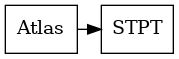
An example task of 3D to 3D mapping between an atlas and a Serial Two Photon Tomography dataset.

Example workflow: Alternating sections to atlases

A typical example is to image a mouse brain using serial sections. Alternate sections are stained for Nissl, or for a specific fluorescent tracer. The pipeline will rigidly register fluorescent slices to neighboring Nissl slices, and will deformably register the Allen CCF Nissl atlas onto the 3D stack of Nissl slices. This allows us to map the anatomical labels from the atlas onto our slices. On each slice, we can quantify cell counts or fluorescence in atlas regions. In 3D we can quantify tracer or cell density.

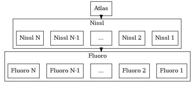
We map our 3D atlas onto a series of 2D nissl images. We also map our 2D Nissl images to their nearest fluorescent image

Note that any time our pipeline registers a 3D volume to a set of 2D slices, a new space is automatically created called a “registered” space. In this space, all the Nissl sections will be rigidly aligned into a 3D reconstruction.

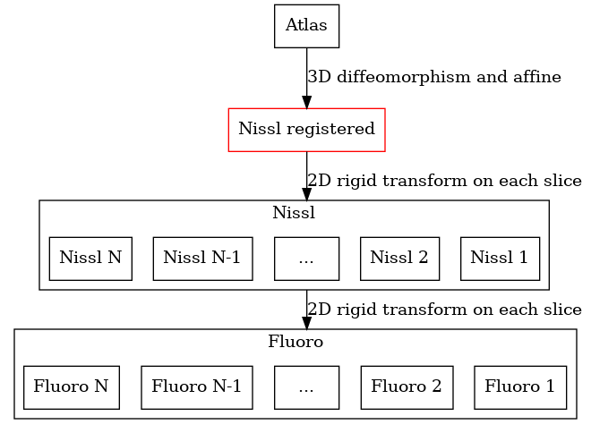
For any 3D to 2D map, a registered space is automatically created (shown in red). No input data is associated with this space, but images can be reconstructed into this space.

Example workflow: Ex vivo MRI

Another example is when MRI is available for a specimen. We typically have an in vivo MRI, ex vivo MRI, and serial section microscopy. The registration tasks are: i) ex vivo to in vivo, ii) ex vivo to serial sections, iii) ex vivo to atlas. We may wish to reconstruct our data in any of the three spaces (in vivo, ex vivo, or atlas). Here the ex vivo MRI plays the role of a common space that is mapped to everything.

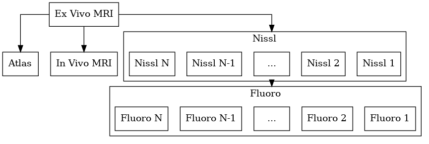
We may also include in vivo and ex vivo mri.

Again, a reconstructed space will be automatically created.

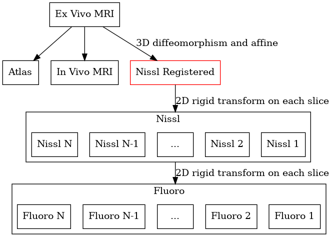
For any 3D to 2D map, a registered space is automatically created (shown in red). No input data is associated with this space, but images can be reconstructed into this space.

Example workflow: Arbitrary layout

In general, a registration task can be formulated by a directed acyclic graph. Each node in the graph is a “space”, which may have more than one image associated with it. Each arrow in the graph is a registration task.

We have built infrastructure to perform necessary maps, and compose transforms to reconstruct any dataset in any space.